



\(\overline{B}^0\to D^{*+}\pi^-\pi^0\) with a spin-1 daughter#

This report implements \(\overline{B}^0\to D^{*+}\pi^-\pi^0\) with a stable spin-1 \(D^{*+}\) in AmpForm-DPD, and the four-body decay \(\overline{B}^0\to D^0\pi^+\pi^-\pi^0\) through \(D^{*+}\to D^0\pi^+\) in AmpForm. Both models use decay chains from QRules and are evaluated with TensorWaves.

The comparisons below use illustrative couplings to check mass projections and helicity correlations.

Hide code cell source

import logging
import os
import warnings
from importlib.metadata import version

import ampform
import attrs
import matplotlib.pyplot as plt
import numpy as np
import phasespace
import qrules
import sympy as sp
from ampform.dynamics.builder import create_relativistic_breit_wigner_with_ff
from ampform.dynamics.form_factor import FormFactor
from ampform.io import aslatex
from ampform_dpd import DalitzPlotDecompositionBuilder
from ampform_dpd.adapter.qrules import normalize_state_ids, to_three_body_decay
from ampform_dpd.dynamics.builder import formulate_breit_wigner_with_form_factor
from ampform_dpd.io import as_markdown_table
from IPython.display import Markdown, Math
from matplotlib.colors import LogNorm
from matplotlib_inline.backend_inline import set_matplotlib_formats
from qrules.io import asmermaid
from qrules.particle import Parity
from qrules.transition import InteractionType, ReactionInfo, StateTransitionManager
from sympy.physics.quantum.cg import CG
from tensorwaves.data.transform import SympyDataTransformer
from tensorwaves.function.sympy import create_parametrized_function

os.environ["TF_CPP_MIN_LOG_LEVEL"] = "3"


set_matplotlib_formats("svg")
logging.getLogger("qrules").setLevel(logging.ERROR)
for package in ("qrules", "ampform", "ampform-dpd", "tensorwaves", "phasespace"):
    print(f"{package}: {version(package)}")
qrules: 0.10.13
ampform: 0.16.1
ampform-dpd: 0.2.4
tensorwaves: 0.4.17
phasespace: 1.10.4

Narrow-width approximation#

The three-body model holds the \(D^{*+}\) at its pole mass. Its width-to-mass ratio is much smaller than those of the other resonances:

Hide code cell source

widths = {
    R"D^{*}(2010)^{+}": (2.01027, 83.4e-6),
    "D_1(2420)": (2.4221, 31.3e-3),
    R"D_2^{*}(2460)": (2.4611, 47.3e-3),
    R"\rho(770)": (0.77511, 149.1e-3),
}
rows = [
    R"| resonance | $m$ [GeV] | $\Gamma$ [GeV] | $\Gamma/m$ |",
    "|---|---:|---:|---:|",
]
rows += [
    f"| ${name}$ | {mass:.5g} | {width:.4g} | {width / mass:.1e} |"
    for name, (mass, width) in widths.items()
]
Markdown("\n".join(rows))

resonance

\(m\) [GeV]

\(\Gamma\) [GeV]

\(\Gamma/m\)

\(D^{*}(2010)^{+}\)

2.0103

8.34e-05

4.1e-05

\(D_1(2420)\)

2.4221

0.0313

1.3e-02

\(D_2^{*}(2460)\)

2.4611

0.0473

1.9e-02

\(\rho(770)\)

0.77511

0.1491

1.9e-01

The measured \(D^{*+}\) width is \(83.4\pm1.8\;\mathrm{keV}\) [BaBar Collaboration, 2013]. The three-body model sums over its helicity, while the four-body model retains its decay angles.

Decay chains for the three-body model#

Label \(\overline{B}^0\) by 0 and \((D^{*+},\pi^-,\pi^0)\) by \((1,2,3)\), so that the Dalitz-plot decomposition variables are

\[\sigma_1=m^2(\pi^-\pi^0),\qquad \sigma_2=m^2(D^{*+}\pi^0),\qquad \sigma_3=m^2(D^{*+}\pi^-).\]

The model includes \(\rho(770)^-\) in \(\sigma_1\), the charged \(D^{**+}\) states in \(\sigma_2\), and the neutral \(D^{**0}\) states in \(\sigma_3\). It retains the two narrow \(P\)-wave charm states, \(D_1(2420)\) and \(D_2^*(2460)\), in both charge configurations. The broad \(D_1(2430)\) is left out because QRules only carries its neutral charge state, which would break the isospin symmetry of the model. Unlike TR-036, there are no identical particles here, so no Bose symmetrization is needed.

The particle database lacks parity for \(D_1(2420)^\pm\); load_particles() assigns \(J^P=1^+\) from the neutral partners. QRules allows strong and weak interactions to accommodate the weak \(\overline{B}^0\) vertex. The filter then selects \(P\)-wave \(\rho(770)^-\to\pi^-\pi^0\) and \(D\)-wave \(D^{**}\to D^{*+}\pi\) decays.

Hide code cell source

DECAY_WAVE = {
    "rho(770)-": 1,
    "D(1)(2420)0": 2,
    "D(1)(2420)+": 2,
    "D(2)*(2460)0": 2,
    "D(2)*(2460)+": 2,
}


def load_particles():
    particle_db = qrules.particle.load_pdg()
    for name in ("D(1)(2420)+", "D(1)(2420)-"):
        particle = particle_db[name]
        assert particle.parity is None
        particle_db.remove(name)
        particle_db.add(attrs.evolve(particle, parity=Parity(+1)))
    return particle_db


def has_physical_decay_wave(transition, node_id):
    (resonance,) = transition.intermediate_states.values()
    return (
        transition.interactions[node_id].l_magnitude
        == DECAY_WAVE[resonance.particle.name]
    )


reaction = qrules.generate_transitions(
    initial_state="B~0",
    final_state=["D*(2010)+", "pi-", "pi0"],
    allowed_intermediate_particles=list(DECAY_WAVE),
    allowed_interaction_types=["strong", "weak"],
    formalism="canonical-helicity",
    particle_db=load_particles(),
    number_of_threads=1,
)
reaction = ReactionInfo(
    [t for t in reaction.transitions if has_physical_decay_wave(t, node_id=1)],
    reaction.formalism,
)
decay = to_three_body_decay(normalize_state_ids(reaction).transitions, min_ls=True)
assert [decay.states[i].name for i in range(4)] == ["B~0", "D*(2010)+", "pi-", "pi0"]
assert {chain.resonance.name for chain in decay.chains} == set(DECAY_WAVE)
resonances = {chain.resonance.name: chain.resonance for chain in decay.chains}
subsystem_ids = {chain.resonance.name: chain.spectator.index for chain in decay.chains}
Markdown(as_markdown_table(decay))

resonance

\(J^P\)

mass (MeV)

width (MeV)

\(L_\mathrm{dec}^\mathrm{min}\)

\(L_\mathrm{prod}^\mathrm{min}\)

\(D_{1}(2420)^{+} \to D^{*}(2010)^{+} \pi^{0}\)

\(1^+\)

2,422

31

2

1

\(D_{1}(2420)^{0} \to D^{*}(2010)^{+} \pi^{-}\)

\(1^+\)

2,422

31

2

1

\(D_{2}^{*}(2460)^{+} \to D^{*}(2010)^{+} \pi^{0}\)

\(2^+\)

2,461

47

2

2

\(D_{2}^{*}(2460)^{0} \to D^{*}(2010)^{+} \pi^{-}\)

\(2^+\)

2,461

47

2

2

\(\rho(770)^{-} \to \pi^{-} \pi^{0}\)

\(1^-\)

775

149

1

0

Hide code cell source

mermaid = asmermaid(
    normalize_state_ids(reaction),
    collapse_graphs=True,
    markdown=True,
)
Markdown(mermaid)
        flowchart LR
    T0_N0["$$\overline{B}^{0}$$"]
    T0_1["$$1: D^{*}(2010)^{+}$$"]
    T0_2["$$2: \pi^{-}$$"]
    T0_3["$$3: \pi^{0}$$"]
    T0_N1@{ shape: text, label: " " }
    T0_4("$$\begin{gathered} D_{1}(2420)^{0} \\\ D_{2}^{*}(2460)^{0} \end{gathered}$$")
    T0_N0 --- T0_4
    T0_4 --- T0_N1
    T0_N0 --- T0_3
    T0_N1 --- T0_1
    T0_N1 --- T0_2
    T1_N0["$$\overline{B}^{0}$$"]
    T1_1["$$1: D^{*}(2010)^{+}$$"]
    T1_2["$$2: \pi^{-}$$"]
    T1_3["$$3: \pi^{0}$$"]
    T1_N1@{ shape: text, label: " " }
    T1_4("$$\begin{gathered} D_{1}(2420)^{+} \\\ D_{2}^{*}(2460)^{+} \end{gathered}$$")
    T1_N0 --- T1_4
    T1_4 --- T1_N1
    T1_N0 --- T1_2
    T1_N1 --- T1_1
    T1_N1 --- T1_3
    T2_N0["$$\overline{B}^{0}$$"]
    T2_1["$$1: D^{*}(2010)^{+}$$"]
    T2_2["$$2: \pi^{-}$$"]
    T2_3["$$3: \pi^{0}$$"]
    T2_N1@{ shape: text, label: " " }
    T2_4("$$\rho(770)^{-}$$")
    T2_N0 --- T2_4
    T2_4 --- T2_N1
    T2_N0 --- T2_1
    T2_N1 --- T2_2
    T2_N1 --- T2_3
    

Three-body amplitude with AmpForm-DPD#

The Dalitz-plot decomposition [Mikhasenko et al., 2020] rotates each decay chain into a common frame. The spin-1 \(D^{*+}\) requires the alignment angles \(\zeta^1_{k(1)}\) shown below.

Each resonance uses a Breit-Wigner dynamics builder. AmpForm-DPD v0.2.4 passes \(\sigma_k^2\) to the decay form factor and the pole mass \(m_R\) as the production daughter mass. The correction below replaces these with \(\sigma_k\) and \(\sqrt{\sigma_k}\) for the resonance’s subsystem.

Hide code cell source

sigma1, sigma2, sigma3 = sigmas = sp.symbols("sigma1:4", nonnegative=True)
m0, m1, m2, m3 = sp.symbols("m0:4", nonnegative=True)

builder = DalitzPlotDecompositionBuilder(decay)
for chain in decay.chains:
    builder.dynamics_choices.register_builder(
        chain.resonance.name, formulate_breit_wigner_with_form_factor
    )
model = builder.formulate(
    reference_subsystem=1, cleanup_summations=True, use_coefficients=True
)

running_mass = {
    f"m_{{{chain.resonance.latex}}}": sigmas[chain.spectator.index - 1]
    for chain in decay.chains
}
form_factor_corrections = {}
for expression in model.amplitudes.values():
    for ff in expression.atoms(FormFactor):
        if ff.s in {s**2 for s in sigmas}:
            form_factor_corrections[ff] = FormFactor(
                sp.sqrt(ff.s), ff.m1, ff.m2, ff.angular_momentum, ff.meson_radius
            )
        elif ff.s == m0**2 and str(ff.m1) in running_mass:
            form_factor_corrections[ff] = FormFactor(
                m0**2,
                sp.sqrt(running_mass[str(ff.m1)]),
                ff.m2,
                ff.angular_momentum,
                ff.meson_radius,
            )
model.amplitudes.update({
    symbol: expression.xreplace(form_factor_corrections)
    for symbol, expression in model.amplitudes.items()
})
for expression in model.amplitudes.values():
    for ff in expression.atoms(FormFactor):
        assert ff.s in set(sigmas) | {m0**2}
        if ff.s == m0**2:
            assert isinstance(ff.m1, sp.Pow)
Math(aslatex(model.amplitudes, terms_per_line=1))
\[\begin{split}\displaystyle \begin{aligned} {A^{1}}_{0,-1,0,0} \;&=\; \sum_{\lambda_{R}=-1}^{1}{\delta_{0, \lambda_{R} + 1} \mathcal{F}_{0}\left(m_{0}^{2}, \sqrt{\sigma_{1}}, m_{D^{*}(2010)^{+}}\right) \mathcal{F}_{1}\left(\sigma_{1}, m_{\pi^{-}}, m_{\pi^{0}}\right) {\mathcal{H}^\mathrm{\rho(770)^{-}}}_{\lambda_{R},-1,0,0} \mathcal{R}_{1}\left(\sigma_{1}, m_{\rho(770)^{-}}, \Gamma_{\rho(770)^{-}}\right) d^{1}_{\lambda_{R},0}\left(\theta_{23}\right)} \\ {A^{2}}_{0,-1,0,0} \;&=\; \sum_{\lambda_{R}=-1}^{1}{\delta_{0 \lambda_{R}} \mathcal{F}_{1}\left(m_{0}^{2}, \sqrt{\sigma_{2}}, m_{\pi^{-}}\right) \mathcal{F}_{2}\left(\sigma_{2}, m_{D^{*}(2010)^{+}}, m_{\pi^{0}}\right) {\mathcal{H}^\mathrm{D_{1}(2420)^{+}}}_{\lambda_{R},0,0,-1} \mathcal{R}_{2}\left(\sigma_{2}, m_{D_{1}(2420)^{+}}, \Gamma_{D_{1}(2420)^{+}}\right) d^{1}_{\lambda_{R},1}\left(\theta_{31}\right)} \\ \;&+\; \sum_{\lambda_{R}=-2}^{2}{\delta_{0 \lambda_{R}} \mathcal{F}_{2}\left(m_{0}^{2}, \sqrt{\sigma_{2}}, m_{\pi^{-}}\right) \mathcal{F}_{2}\left(\sigma_{2}, m_{D^{*}(2010)^{+}}, m_{\pi^{0}}\right) {\mathcal{H}^\mathrm{D_{2}^{*}(2460)^{+}}}_{\lambda_{R},0,0,-1} \mathcal{R}_{2}\left(\sigma_{2}, m_{D_{2}^{*}(2460)^{+}}, \Gamma_{D_{2}^{*}(2460)^{+}}\right) d^{2}_{\lambda_{R},1}\left(\theta_{31}\right)} \\ {A^{3}}_{0,-1,0,0} \;&=\; \sum_{\lambda_{R}=-1}^{1}{\delta_{0 \lambda_{R}} \mathcal{F}_{1}\left(m_{0}^{2}, \sqrt{\sigma_{3}}, m_{\pi^{0}}\right) \mathcal{F}_{2}\left(\sigma_{3}, m_{D^{*}(2010)^{+}}, m_{\pi^{-}}\right) {\mathcal{H}^\mathrm{D_{1}(2420)^{0}}}_{\lambda_{R},0,-1,0} \mathcal{R}_{2}\left(\sigma_{3}, m_{D_{1}(2420)^{0}}, \Gamma_{D_{1}(2420)^{0}}\right) d^{1}_{\lambda_{R},-1}\left(\theta_{12}\right)} \\ \;&+\; \sum_{\lambda_{R}=-2}^{2}{\delta_{0 \lambda_{R}} \mathcal{F}_{2}\left(m_{0}^{2}, \sqrt{\sigma_{3}}, m_{\pi^{0}}\right) \mathcal{F}_{2}\left(\sigma_{3}, m_{D^{*}(2010)^{+}}, m_{\pi^{-}}\right) {\mathcal{H}^\mathrm{D_{2}^{*}(2460)^{0}}}_{\lambda_{R},0,-1,0} \mathcal{R}_{2}\left(\sigma_{3}, m_{D_{2}^{*}(2460)^{0}}, \Gamma_{D_{2}^{*}(2460)^{0}}\right) d^{2}_{\lambda_{R},-1}\left(\theta_{12}\right)} \\ {A^{1}}_{0,0,0,0} \;&=\; \sum_{\lambda_{R}=-1}^{1}{- \delta_{0 \lambda_{R}} \mathcal{F}_{0}\left(m_{0}^{2}, \sqrt{\sigma_{1}}, m_{D^{*}(2010)^{+}}\right) \mathcal{F}_{1}\left(\sigma_{1}, m_{\pi^{-}}, m_{\pi^{0}}\right) {\mathcal{H}^\mathrm{\rho(770)^{-}}}_{\lambda_{R},0,0,0} \mathcal{R}_{1}\left(\sigma_{1}, m_{\rho(770)^{-}}, \Gamma_{\rho(770)^{-}}\right) d^{1}_{\lambda_{R},0}\left(\theta_{23}\right)} \\ {A^{2}}_{0,0,0,0} \;&=\; \sum_{\lambda_{R}=-1}^{1}{- \delta_{0 \lambda_{R}} \mathcal{F}_{1}\left(m_{0}^{2}, \sqrt{\sigma_{2}}, m_{\pi^{-}}\right) \mathcal{F}_{2}\left(\sigma_{2}, m_{D^{*}(2010)^{+}}, m_{\pi^{0}}\right) {\mathcal{H}^\mathrm{D_{1}(2420)^{+}}}_{\lambda_{R},0,0,0} \mathcal{R}_{2}\left(\sigma_{2}, m_{D_{1}(2420)^{+}}, \Gamma_{D_{1}(2420)^{+}}\right) d^{1}_{\lambda_{R},0}\left(\theta_{31}\right)} \\ \;&+\; \sum_{\lambda_{R}=-2}^{2}{- \delta_{0 \lambda_{R}} \mathcal{F}_{2}\left(m_{0}^{2}, \sqrt{\sigma_{2}}, m_{\pi^{-}}\right) \mathcal{F}_{2}\left(\sigma_{2}, m_{D^{*}(2010)^{+}}, m_{\pi^{0}}\right) {\mathcal{H}^\mathrm{D_{2}^{*}(2460)^{+}}}_{\lambda_{R},0,0,0} \mathcal{R}_{2}\left(\sigma_{2}, m_{D_{2}^{*}(2460)^{+}}, \Gamma_{D_{2}^{*}(2460)^{+}}\right) d^{2}_{\lambda_{R},0}\left(\theta_{31}\right)} \\ {A^{3}}_{0,0,0,0} \;&=\; \sum_{\lambda_{R}=-1}^{1}{\delta_{0 \lambda_{R}} \mathcal{F}_{1}\left(m_{0}^{2}, \sqrt{\sigma_{3}}, m_{\pi^{0}}\right) \mathcal{F}_{2}\left(\sigma_{3}, m_{D^{*}(2010)^{+}}, m_{\pi^{-}}\right) {\mathcal{H}^\mathrm{D_{1}(2420)^{0}}}_{\lambda_{R},0,0,0} \mathcal{R}_{2}\left(\sigma_{3}, m_{D_{1}(2420)^{0}}, \Gamma_{D_{1}(2420)^{0}}\right) d^{1}_{\lambda_{R},0}\left(\theta_{12}\right)} \\ \;&+\; \sum_{\lambda_{R}=-2}^{2}{\delta_{0 \lambda_{R}} \mathcal{F}_{2}\left(m_{0}^{2}, \sqrt{\sigma_{3}}, m_{\pi^{0}}\right) \mathcal{F}_{2}\left(\sigma_{3}, m_{D^{*}(2010)^{+}}, m_{\pi^{-}}\right) {\mathcal{H}^\mathrm{D_{2}^{*}(2460)^{0}}}_{\lambda_{R},0,0,0} \mathcal{R}_{2}\left(\sigma_{3}, m_{D_{2}^{*}(2460)^{0}}, \Gamma_{D_{2}^{*}(2460)^{0}}\right) d^{2}_{\lambda_{R},0}\left(\theta_{12}\right)} \\ {A^{1}}_{0,1,0,0} \;&=\; \sum_{\lambda_{R}=-1}^{1}{\delta_{0, \lambda_{R} - 1} \mathcal{F}_{0}\left(m_{0}^{2}, \sqrt{\sigma_{1}}, m_{D^{*}(2010)^{+}}\right) \mathcal{F}_{1}\left(\sigma_{1}, m_{\pi^{-}}, m_{\pi^{0}}\right) {\mathcal{H}^\mathrm{\rho(770)^{-}}}_{\lambda_{R},1,0,0} \mathcal{R}_{1}\left(\sigma_{1}, m_{\rho(770)^{-}}, \Gamma_{\rho(770)^{-}}\right) d^{1}_{\lambda_{R},0}\left(\theta_{23}\right)} \\ {A^{2}}_{0,1,0,0} \;&=\; \sum_{\lambda_{R}=-1}^{1}{\delta_{0 \lambda_{R}} \mathcal{F}_{1}\left(m_{0}^{2}, \sqrt{\sigma_{2}}, m_{\pi^{-}}\right) \mathcal{F}_{2}\left(\sigma_{2}, m_{D^{*}(2010)^{+}}, m_{\pi^{0}}\right) {\mathcal{H}^\mathrm{D_{1}(2420)^{+}}}_{\lambda_{R},0,0,1} \mathcal{R}_{2}\left(\sigma_{2}, m_{D_{1}(2420)^{+}}, \Gamma_{D_{1}(2420)^{+}}\right) d^{1}_{\lambda_{R},-1}\left(\theta_{31}\right)} \\ \;&+\; \sum_{\lambda_{R}=-2}^{2}{\delta_{0 \lambda_{R}} \mathcal{F}_{2}\left(m_{0}^{2}, \sqrt{\sigma_{2}}, m_{\pi^{-}}\right) \mathcal{F}_{2}\left(\sigma_{2}, m_{D^{*}(2010)^{+}}, m_{\pi^{0}}\right) {\mathcal{H}^\mathrm{D_{2}^{*}(2460)^{+}}}_{\lambda_{R},0,0,1} \mathcal{R}_{2}\left(\sigma_{2}, m_{D_{2}^{*}(2460)^{+}}, \Gamma_{D_{2}^{*}(2460)^{+}}\right) d^{2}_{\lambda_{R},-1}\left(\theta_{31}\right)} \\ {A^{3}}_{0,1,0,0} \;&=\; \sum_{\lambda_{R}=-1}^{1}{\delta_{0 \lambda_{R}} \mathcal{F}_{1}\left(m_{0}^{2}, \sqrt{\sigma_{3}}, m_{\pi^{0}}\right) \mathcal{F}_{2}\left(\sigma_{3}, m_{D^{*}(2010)^{+}}, m_{\pi^{-}}\right) {\mathcal{H}^\mathrm{D_{1}(2420)^{0}}}_{\lambda_{R},0,1,0} \mathcal{R}_{2}\left(\sigma_{3}, m_{D_{1}(2420)^{0}}, \Gamma_{D_{1}(2420)^{0}}\right) d^{1}_{\lambda_{R},1}\left(\theta_{12}\right)} \\ \;&+\; \sum_{\lambda_{R}=-2}^{2}{\delta_{0 \lambda_{R}} \mathcal{F}_{2}\left(m_{0}^{2}, \sqrt{\sigma_{3}}, m_{\pi^{0}}\right) \mathcal{F}_{2}\left(\sigma_{3}, m_{D^{*}(2010)^{+}}, m_{\pi^{-}}\right) {\mathcal{H}^\mathrm{D_{2}^{*}(2460)^{0}}}_{\lambda_{R},0,1,0} \mathcal{R}_{2}\left(\sigma_{3}, m_{D_{2}^{*}(2460)^{0}}, \Gamma_{D_{2}^{*}(2460)^{0}}\right) d^{2}_{\lambda_{R},1}\left(\theta_{12}\right)} \\ \end{aligned}\end{split}\]

The nine amplitude components correspond to three \(D^{*+}\) helicities per subsystem. The scattering and alignment angles are:

Hide code cell source

x, y, z = sp.symbols("x y z", real=True)
kinematics = {
    symbol: expression
    for symbol, expression in model.variables.items()
    if str(symbol).startswith(("theta", R"\zeta"))
}
Math(aslatex(kinematics))
\[\begin{split}\displaystyle \begin{aligned} \theta_{23} \;&=\; \operatorname{acos}{\left(\frac{2 \sigma_{1} \left(- m_{1}^{2} - m_{2}^{2} + \sigma_{3}\right) - \left(m_{0}^{2} - m_{1}^{2} - \sigma_{1}\right) \left(m_{2}^{2} - m_{3}^{2} + \sigma_{1}\right)}{\sqrt{\lambda\left(m_{0}^{2}, m_{1}^{2}, \sigma_{1}\right)} \sqrt{\lambda\left(\sigma_{1}, m_{2}^{2}, m_{3}^{2}\right)}} \right)} \\ \theta_{31} \;&=\; \operatorname{acos}{\left(\frac{2 \sigma_{2} \left(- m_{2}^{2} - m_{3}^{2} + \sigma_{1}\right) - \left(m_{0}^{2} - m_{2}^{2} - \sigma_{2}\right) \left(- m_{1}^{2} + m_{3}^{2} + \sigma_{2}\right)}{\sqrt{\lambda\left(m_{0}^{2}, m_{2}^{2}, \sigma_{2}\right)} \sqrt{\lambda\left(\sigma_{2}, m_{3}^{2}, m_{1}^{2}\right)}} \right)} \\ \theta_{12} \;&=\; \operatorname{acos}{\left(\frac{2 \sigma_{3} \left(- m_{1}^{2} - m_{3}^{2} + \sigma_{2}\right) - \left(m_{0}^{2} - m_{3}^{2} - \sigma_{3}\right) \left(m_{1}^{2} - m_{2}^{2} + \sigma_{3}\right)}{\sqrt{\lambda\left(m_{0}^{2}, m_{3}^{2}, \sigma_{3}\right)} \sqrt{\lambda\left(\sigma_{3}, m_{1}^{2}, m_{2}^{2}\right)}} \right)} \\ \zeta^1_{1(1)} \;&=\; 0 \\ \zeta^1_{2(1)} \;&=\; \operatorname{acos}{\left(\frac{2 m_{1}^{2} \left(- m_{0}^{2} - m_{3}^{2} + \sigma_{3}\right) + \left(m_{0}^{2} + m_{1}^{2} - \sigma_{1}\right) \left(- m_{1}^{2} - m_{3}^{2} + \sigma_{2}\right)}{\sqrt{\lambda\left(m_{0}^{2}, m_{1}^{2}, \sigma_{1}\right)} \sqrt{\lambda\left(\sigma_{2}, m_{1}^{2}, m_{3}^{2}\right)}} \right)} \\ \zeta^1_{3(1)} \;&=\; - \operatorname{acos}{\left(\frac{2 m_{1}^{2} \left(- m_{0}^{2} - m_{2}^{2} + \sigma_{2}\right) + \left(m_{0}^{2} + m_{1}^{2} - \sigma_{1}\right) \left(- m_{1}^{2} - m_{2}^{2} + \sigma_{3}\right)}{\sqrt{\lambda\left(m_{0}^{2}, m_{1}^{2}, \sigma_{1}\right)} \sqrt{\lambda\left(\sigma_{3}, m_{1}^{2}, m_{2}^{2}\right)}} \right)} \\ \end{aligned}\end{split}\]

Helicity couplings of a spin-1 daughter#

With a spin-1 daughter, one complex coupling per decay chain is no longer enough: each chain comes with a coupling \(\mathcal{H}^R_\lambda\) for every \(D^{*+}\) helicity \(\lambda\in\{-1,0,+1\}\), fifteen in total. They are not independent. The \(\overline{B}^0\) vertex is weak, so parity constrains nothing there, but the resonance decays are strong, and the single decay wave selected above fixes the helicity pattern up to one overall coupling per resonance.

For \(R\to D^{*+}\pi\) in a \(D\) wave, the pattern is the Clebsch-Gordan coefficient \(\langle L\,0;S\,\lambda\mid J_R\,\lambda\rangle\) with \(L=2\) and \(S=1\):

\[\mathcal{H}^R_\lambda \propto \langle 2\,0;1\,\lambda\mid J_R\,\lambda\rangle .\]

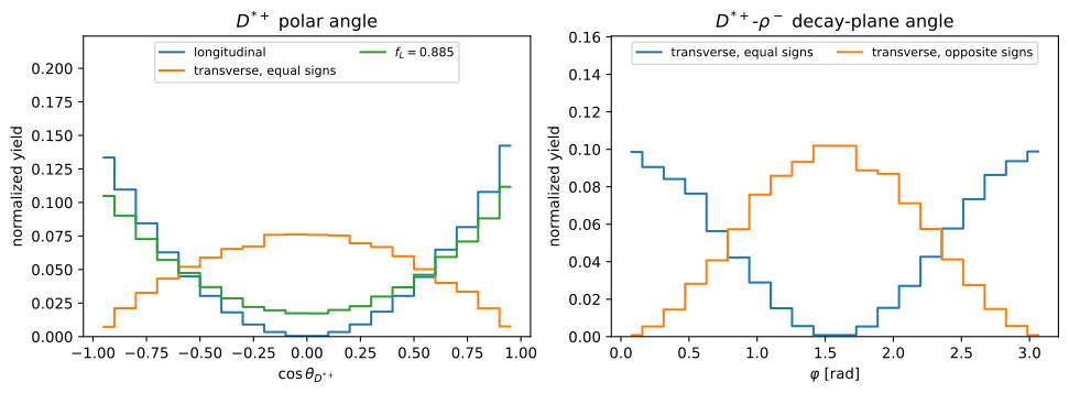
For \(J_R=1\) this is even in \(\lambda\); for \(J_R=2\) it is odd, and \(\langle2\,0;1\,0\mid2\,0\rangle=0\) makes the \(D_2^*(2460)\) longitudinal coupling vanish outright. The same conclusion follows from the parity relation \(\mathcal{H}_{-\lambda}=P_R(-1)^{J_R-1}\mathcal{H}_{\lambda}\). For \(\overline{B}^0\to D^{*+}\rho^-\), on the other hand, all three couplings are free: this is the vector-vector configuration whose longitudinal fraction \(f_L\) is the quantity experiments quote. We take \(f_L=0.885\) and split the transverse strength equally.

That leaves seven free complex numbers, one per resonance plus two extra for the \(\rho^-\) polarization, which is exactly the number of independent \(LS\) couplings in the canonical basis.

Hide code cell source

HELICITY_SLOT = {1: 1, 2: 3, 3: 2}
LONGITUDINAL_FRACTION = 0.885


def coupling_symbol(resonance_name, helicity):
    resonance = resonances[resonance_name]
    subsystem = subsystem_ids[resonance_name]
    indices = [0, 0, 0, 0]
    indices[HELICITY_SLOT[subsystem]] = helicity
    if subsystem == 1:
        indices[0] = helicity
    base = sp.IndexedBase(Rf"\mathcal{{H}}^\mathrm{{{resonance.latex}}}")
    return base[tuple(indices)]


def decay_wave_pattern(resonance_name):
    spin = resonances[resonance_name].spin
    wave = DECAY_WAVE[resonance_name]
    return {
        helicity: float(CG(wave, 0, 1, helicity, spin, helicity).doit())
        for helicity in (-1, 0, 1)
    }


transverse = np.sqrt((1 / LONGITUDINAL_FRACTION - 1) / 2)
patterns = {
    name: {-1: transverse, 0: 1.0, +1: transverse}
    if subsystem_ids[name] == 1
    else decay_wave_pattern(name)
    for name in DECAY_WAVE
}
assert patterns["D(2)*(2460)0"][0] == 0
assert patterns["D(1)(2420)0"][-1] == patterns["D(1)(2420)0"][+1]
rows = [
    R"| resonance | $\lambda=-1$ | $\lambda=0$ | $\lambda=+1$ |",
    "|---|---:|---:|---:|",
]
rows += [
    f"| ${resonances[name].latex}$ | "
    + " | ".join(f"{pattern[h]:+.4f}" for h in (-1, 0, 1))
    + " |"
    for name, pattern in patterns.items()
]
Markdown("\n".join(rows))

resonance

\(\lambda=-1\)

\(\lambda=0\)

\(\lambda=+1\)

\(\rho(770)^{-}\)

+0.2549

+1.0000

+0.2549

\(D_{1}(2420)^{0}\)

+0.3162

-0.6325

+0.3162

\(D_{1}(2420)^{+}\)

+0.3162

-0.6325

+0.3162

\(D_{2}^{*}(2460)^{0}\)

+0.7071

+0.0000

-0.7071

\(D_{2}^{*}(2460)^{+}\)

+0.7071

+0.0000

-0.7071

The couplings themselves are set from illustrative component fractions. As in TR-036 the fractions are defined through the diagonal integrals \(N_R=\int_\mathcal{D}I_R\,\mathrm{d}\sigma_3\,\mathrm{d}\sigma_1\) of each component evaluated on its own, so that the numbers mean the same thing for every lineshape. Three-body phase space is flat in \(\mathrm{d}\sigma_3\,\mathrm{d}\sigma_1\) for a scalar parent, so no extra momentum weight is needed.

Hide code cell source

expression = model.full_expression.xreplace(model.variables).doit()
expression = expression.xreplace(model.masses)
couplings = {
    symbol: value
    for symbol, value in model.parameter_defaults.items()
    if isinstance(symbol, sp.Indexed)
}
fixed_parameters = {
    symbol: value
    for symbol, value in model.parameter_defaults.items()
    if symbol not in couplings
}
expression = expression.xreplace(fixed_parameters)
assert set(couplings) == {coupling_symbol(n, h) for n in DECAY_WAVE for h in (-1, 0, 1)}
intensity_function = create_parametrized_function(expression, couplings, backend="jax")

MASSES = [float(model.masses[sp.Symbol(f"m{i}", nonnegative=True)]) for i in range(4)]
SIGMA_SUM = sum(mass**2 for mass in MASSES)


def set_couplings(scales):
    parameters = {}
    for name, pattern in patterns.items():
        for helicity, weight in pattern.items():
            symbol = str(coupling_symbol(name, helicity))
            parameters[symbol] = complex(scales.get(name, 0)) * weight
    intensity_function.update_parameters(parameters)


def evaluate(scales, data):
    set_couplings(scales)
    return np.asarray(intensity_function(data))

Physical region and the Dalitz plot#

The physical region follows from the Kibble function \(\phi<0\) [Byckling and Kajantie, 1973], evaluated on a regular grid in \(\left(\sigma_3,\sigma_1\right)\).

Hide code cell source

def kallen(x, y, z):
    return x**2 + y**2 + z**2 - 2 * (x * y + y * z + z * x)


def is_inside(s1, s2, s3):
    parent = MASSES[0] ** 2
    return (
        kallen(
            kallen(s2, MASSES[2] ** 2, parent),
            kallen(s3, MASSES[3] ** 2, parent),
            kallen(s1, MASSES[1] ** 2, parent),
        )
        < 0
    )


def dalitz_grid(n_bins):
    parent, m_dstar, m_pim, m_pi0 = MASSES
    x_edges = np.linspace((m_dstar + m_pim) ** 2, (parent - m_pi0) ** 2, n_bins + 1)
    y_edges = np.linspace((m_pim + m_pi0) ** 2, (parent - m_dstar) ** 2, n_bins + 1)
    s3, s1 = np.meshgrid(
        (x_edges[1:] + x_edges[:-1]) / 2, (y_edges[1:] + y_edges[:-1]) / 2
    )
    s2 = SIGMA_SUM - s1 - s3
    inside = is_inside(s1, s2, s3)
    data = {"sigma1": s1[inside], "sigma2": s2[inside], "sigma3": s3[inside]}
    cell_area = (x_edges[1] - x_edges[0]) * (y_edges[1] - y_edges[0])
    return x_edges, y_edges, inside, data, cell_area


x_edges, y_edges, inside, grid_data, cell_area = dalitz_grid(500)
norms = {
    name: float(np.sum(evaluate({name: 1.0}, grid_data)) * cell_area)
    for name in DECAY_WAVE
}
assert all(np.isfinite(value) and value > 0 for value in norms.values())
*_, coarse_data, coarse_area = dalitz_grid(250)
coarse_norms = {
    name: float(np.sum(evaluate({name: 1.0}, coarse_data)) * coarse_area)
    for name in DECAY_WAVE
}
grid_stability = max(abs(coarse_norms[name] / norms[name] - 1) for name in norms)
assert grid_stability < 0.02, grid_stability

fractions = {
    "rho(770)-": 0.45,
    "D(2)*(2460)0": 0.20,
    "D(1)(2420)0": 0.15,
    "D(2)*(2460)+": 0.12,
    "D(1)(2420)+": 0.08,
}
phases = {
    "rho(770)-": 0.0,
    "D(2)*(2460)0": 120.0,
    "D(1)(2420)0": -60.0,
    "D(2)*(2460)+": 150.0,
    "D(1)(2420)+": -30.0,
}
scales = {
    name: np.sqrt(fraction / norms[name]) * np.exp(1j * np.deg2rad(phases[name]))
    for name, fraction in fractions.items()
}
density_values = evaluate(scales, grid_data)
coherent_integral = float(np.sum(density_values) * cell_area)
assert np.isfinite(density_values).all()
assert (density_values >= 0).all()
rows = [
    "| resonance | subsystem | input fraction [%] | phase [deg] | model fraction [%] |",
    "|---|---|---:|---:|---:|",
]
for name, fraction in fractions.items():
    model_fraction = abs(scales[name]) ** 2 * norms[name] / coherent_integral
    rows.append(
        f"| ${resonances[name].latex}$ | $\\sigma_{subsystem_ids[name]}$ "
        f"| {100 * fraction:g} | {phases[name]:g} | {100 * model_fraction:.2f} |"
    )
rows.append(
    f"\nLargest change in component integrals on grid refinement: {100 * grid_stability:.2f}%."
)
Markdown("\n".join(rows))

resonance

subsystem

input fraction [%]

phase [deg]

model fraction [%]

\(\rho(770)^{-}\)

\(\sigma_1\)

45

0

44.26

\(D_{2}^{*}(2460)^{0}\)

\(\sigma_3\)

20

120

19.67

\(D_{1}(2420)^{0}\)

\(\sigma_3\)

15

-60

14.75

\(D_{2}^{*}(2460)^{+}\)

\(\sigma_2\)

12

150

11.80

\(D_{1}(2420)^{+}\)

\(\sigma_2\)

8

-30

7.87

Largest change in component integrals on grid refinement: 0.51%.

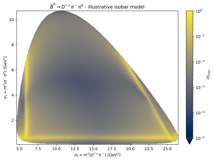
The model fractions differ from the input fractions only through interference, which is why they do not sum to 100%. The Dalitz plot below shows the coherent intensity relative to its maximum.
Hide code cell source

density = np.full(inside.shape, np.nan)
density[inside] = density_values
relative_density = density / np.nanmax(density)

fig, ax = plt.subplots(figsize=(7.5, 5.6), layout="constrained")
mesh = ax.pcolormesh(
    x_edges,
    y_edges,
    np.ma.masked_invalid(relative_density),
    cmap="cividis",
    norm=LogNorm(vmin=1e-5, vmax=1),
    rasterized=True,
)
ax.set(
    xlabel=R"$\sigma_3 = m^2(D^{*+}\pi^-)$ [GeV$^2$]",
    ylabel=R"$\sigma_1 = m^2(\pi^-\pi^0)$ [GeV$^2$]",
    title=R"$\overline{B}^0\to D^{*+}\pi^-\pi^0$ - illustrative isobar model",
)
fig.colorbar(mesh, ax=ax, label=R"$I/I_\mathrm{max}$", extend="min")
fig.savefig("dalitz.svg")
plt.show()
../_images/9c5277b26f95f2c92cb1d3730a354e61273e5eba26292323a0ecdae7427eea35.svg

The three subsystems are cleanly separated: the \(D^{**0}\) states form the vertical band near \(\sigma_3\approx6\;\mathrm{GeV}^2\), the \(\rho(770)^-\) the horizontal band at \(\sigma_1\approx0.6\;\mathrm{GeV}^2\), and the \(D^{**+}\) states the diagonal band of constant \(\sigma_2\).

One-dimensional AmpForm-DPD projections#

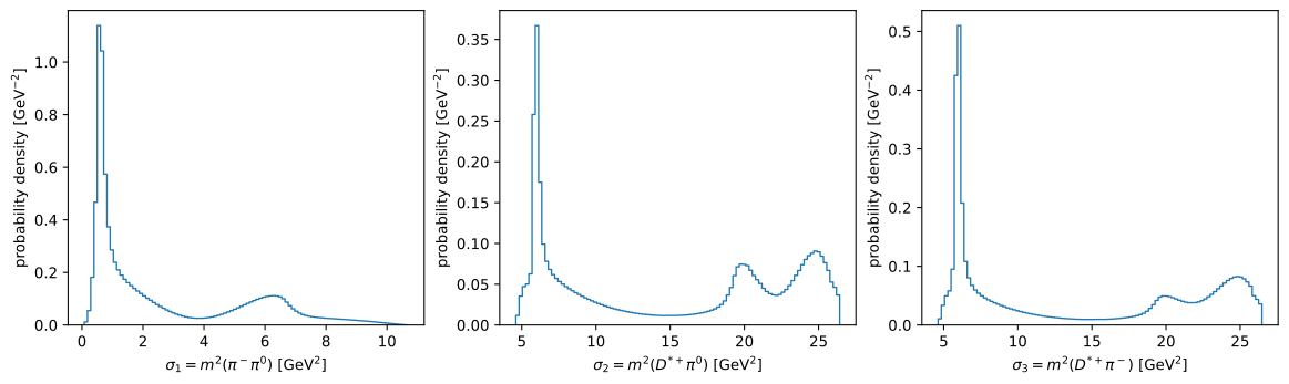
The three pair-mass projections integrate the coherent intensity over the physical Dalitz grid. Each has unit area in \(\sigma_k\); the phase-space measure is constant in \(d\sigma_3\,d\sigma_1\).
Hide code cell source

projection_edges = {
    1: y_edges[::5],
    2: np.linspace((MASSES[1] + MASSES[3]) ** 2, (MASSES[0] - MASSES[2]) ** 2, 101),
    3: x_edges[::5],
}
projection_labels = {
    1: R"$\sigma_1=m^2(\pi^-\pi^0)$ [GeV$^2$]",
    2: R"$\sigma_2=m^2(D^{*+}\pi^0)$ [GeV$^2$]",
    3: R"$\sigma_3=m^2(D^{*+}\pi^-)$ [GeV$^2$]",
}
fig, axes = plt.subplots(1, 3, figsize=(12, 3.5), layout="constrained")
for ax, subsystem in zip(axes, (1, 2, 3), strict=True):
    bin_edges = projection_edges[subsystem]
    projection, _ = np.histogram(
        grid_data[f"sigma{subsystem}"],
        bins=bin_edges,
        weights=density_values * cell_area,
    )
    np.testing.assert_allclose(projection.sum(), coherent_integral, rtol=1e-10)
    projection /= coherent_integral * np.diff(bin_edges)
    ax.stairs(projection, bin_edges)
    ax.set(
        xlabel=projection_labels[subsystem],
        ylabel=R"probability density [GeV$^{-2}$]",
        ylim=(0, None),
    )
fig.savefig("projections-dpd.svg")
plt.show()
../_images/bec35e240819d2256a30e3090971decf8cb0b3c9cc18616613fbd4df9b4a900c.svg

Helicity sums and interference#

The three-body intensity sums incoherently over the \(D^{*+}\) helicity, \(I=\sum_\lambda\left|\sum_R\mathcal{A}^R_\lambda\right|^2\). The check below evaluates \(I_{ab}-I_a-I_b\) for each pair of components at random physical points. With the selected decay waves, opposite helicity-parity patterns cancel pointwise in this sum.

A second check compares longitudinal and transverse \(\rho^-\) couplings. Equal and opposite transverse signs give identical Dalitz densities; longitudinal and transverse configurations give different densities.

Hide code cell source

def sample_physical_region(n_points, seed=37):
    parent, m_dstar, m_pim, m_pi0 = MASSES
    rng = np.random.default_rng(seed)
    collected = {"sigma1": [], "sigma3": []}
    while sum(len(v) for v in collected["sigma1"]) < n_points:
        s3 = rng.uniform((m_dstar + m_pim) ** 2, (parent - m_pi0) ** 2, 20_000)
        s1 = rng.uniform((m_pim + m_pi0) ** 2, (parent - m_dstar) ** 2, 20_000)
        accepted = is_inside(s1, SIGMA_SUM - s1 - s3, s3)
        collected["sigma1"].append(s1[accepted])
        collected["sigma3"].append(s3[accepted])
    s1 = np.concatenate(collected["sigma1"])[:n_points]
    s3 = np.concatenate(collected["sigma3"])[:n_points]
    return {"sigma1": s1, "sigma2": SIGMA_SUM - s1 - s3, "sigma3": s3}


test_data = sample_physical_region(2_000)
helicity_parity = {
    name: "even" if pattern[+1] * pattern[-1] >= 0 else "odd"
    for name, pattern in patterns.items()
}
rows = [
    R"| pair | same $\lambda$-parity | $\left\langle\left|I_{ab}-I_a-I_b\right|\right\rangle/\sqrt{I_aI_b}$ |",
    "|---|:-:|---:|",
]
for i, first in enumerate(DECAY_WAVE):
    for second in list(DECAY_WAVE)[i + 1 :]:
        i_a = evaluate({first: 1.0}, test_data)
        i_b = evaluate({second: 1.0}, test_data)
        cross = evaluate({first: 1.0, second: 1.0}, test_data) - i_a - i_b
        typical = float(np.mean(np.abs(cross) / np.sqrt(i_a * i_b)))
        same = helicity_parity[first] == helicity_parity[second]
        assert typical > 1e-2 if same else typical < 1e-9, (first, second, typical)
        rows.append(
            f"| ${resonances[first].latex}$, ${resonances[second].latex}$ "
            f"| {'yes' if same else 'no'} | {typical:.1e} |"
        )

saved_pattern = patterns["rho(770)-"]
polarization_densities = {}
for label, pattern in (
    ("longitudinal", {-1: 0.0, 0: 1.0, +1: 0.0}),
    ("transverse, equal signs", {-1: 1.0, 0: 0.0, +1: +1.0}),
    ("transverse, opposite signs", {-1: 1.0, 0: 0.0, +1: -1.0}),
):
    patterns["rho(770)-"] = pattern
    values = evaluate({"rho(770)-": 1.0}, test_data)
    polarization_densities[label] = values / values.sum()
patterns["rho(770)-"] = saved_pattern


def relative_difference(first, second):
    return float(
        np.max(np.abs(polarization_densities[first] - polarization_densities[second]))
        / polarization_densities[first].max()
    )


transverse_sign = relative_difference(
    "transverse, equal signs", "transverse, opposite signs"
)
polarization = relative_difference("longitudinal", "transverse, equal signs")
assert transverse_sign == 0, transverse_sign
assert polarization > 0.5, polarization
rows.append(
    "\nRelative difference between the two transverse sign conventions: "
    f"{transverse_sign:.0e}. Between longitudinal and transverse: {100 * polarization:.0f}%."
)
Markdown("\n".join(rows))

| pair | same \(\lambda\)-parity | \(\left\langle\left|I_{ab}-I_a-I_b\right|\right\rangle/\sqrt{I_aI_b}\) | |—|:-:|—:| | \(\rho(770)^{-}\), \(D_{1}(2420)^{0}\) | yes | 8.1e-01 | | \(\rho(770)^{-}\), \(D_{1}(2420)^{+}\) | yes | 8.3e-01 | | \(\rho(770)^{-}\), \(D_{2}^{*}(2460)^{0}\) | no | 2.2e-14 | | \(\rho(770)^{-}\), \(D_{2}^{*}(2460)^{+}\) | no | 4.9e-15 | | \(D_{1}(2420)^{0}\), \(D_{1}(2420)^{+}\) | yes | 1.1e+00 | | \(D_{1}(2420)^{0}\), \(D_{2}^{*}(2460)^{0}\) | no | 6.7e-15 | | \(D_{1}(2420)^{0}\), \(D_{2}^{*}(2460)^{+}\) | no | 4.0e-15 | | \(D_{1}(2420)^{+}\), \(D_{2}^{*}(2460)^{0}\) | no | 5.3e-15 | | \(D_{1}(2420)^{+}\), \(D_{2}^{*}(2460)^{+}\) | no | 5.6e-16 | | \(D_{2}^{*}(2460)^{0}\), \(D_{2}^{*}(2460)^{+}\) | yes | 1.7e+00 |

Relative difference between the two transverse sign conventions: 0e+00. Between longitudinal and transverse: 99%.

Four-body model with AmpForm#

StateTransitionManager.add_final_state_grouping requires \(D^0\) and \(\pi^+\) to share a decay node. Since allowed_intermediate_particles applies to every intermediate edge, keeps_pinned_chain() additionally requires a \(D^{*+}\) and selects the same resonance decay waves as the three-body model, plus a \(P\) wave for \(D^{*+}\to D^0\pi^+\).

All four final-state particles are spinless, so no spin alignment amplitudes are needed.

Hide code cell source

FOUR_BODY_WAVE = {**DECAY_WAVE, "D*(2010)+": 1}


def keeps_pinned_chain(transition):
    names = {state.particle.name for state in transition.intermediate_states.values()}
    if "D*(2010)+" not in names or len(names) != 2:
        return False
    topology = transition.topology
    (initial_edge,) = topology.incoming_edge_ids
    production_node = topology.edges[initial_edge].ending_node_id
    for node_id in topology.nodes:
        if node_id == production_node:
            continue
        (parent,) = topology.get_edge_ids_ingoing_to_node(node_id)
        resonance = transition.states[parent].particle.name
        if transition.interactions[node_id].l_magnitude != FOUR_BODY_WAVE[resonance]:
            return False
    return True


stm = StateTransitionManager(
    initial_state=["B~0"],
    final_state=["D0", "pi+", "pi-", "pi0"],
    allowed_intermediate_particles=list(FOUR_BODY_WAVE),
    formalism="canonical-helicity",
    particle_db=load_particles(),
    max_angular_momentum=2,
    max_spin_magnitude=2,
    number_of_threads=1,
)
stm.add_final_state_grouping([["D0", "pi+"]])
stm.set_allowed_interaction_types([InteractionType.STRONG, InteractionType.WEAK])
four_body_reaction = stm.find_solutions(stm.create_problem_sets())
four_body_reaction = ReactionInfo(
    [t for t in four_body_reaction.transitions if keeps_pinned_chain(t)],
    formalism="helicity",
)
assert len({t.topology for t in four_body_reaction.transitions}) == 3
assert {s.name for s in four_body_reaction.final_state.values()} == {
    "D0",
    "pi+",
    "pi-",
    "pi0",
}
Markdown(
    "The pinned reaction has "
    f"{len(four_body_reaction.transitions)} transitions over three topologies, with intermediate states "
    + ", ".join(
        f"${four_body_reaction.get_intermediate_particles()[n].latex}$"
        for n in sorted(four_body_reaction.get_intermediate_particles().names)
    )
    + "."
)

The pinned reaction has 18 transitions over three topologies, with intermediate states \(D_{1}(2420)^{+}\), \(D_{1}(2420)^{0}\), \(D_{2}^{*}(2460)^{+}\), \(D_{2}^{*}(2460)^{0}\), \(D^{*}(2010)^{+}\), \(\rho(770)^{-}\).

Hide code cell source

mermaid = asmermaid(
    four_body_reaction,
    collapse_graphs=True,
    markdown=True,
)
Markdown(mermaid)
        flowchart LR
    T0_0["$$0: D^{0}$$"]
    T0_1["$$1: \pi^{+}$$"]
    T0_2["$$2: \pi^{-}$$"]
    T0_3["$$3: \pi^{0}$$"]
    T0_N0["$$\overline{B}^{0}$$"]
    T0_N1@{ shape: text, label: " " }
    T0_N2@{ shape: text, label: " " }
    T0_4("$$\begin{gathered} D_{1}(2420)^{0} \\\ D_{2}^{*}(2460)^{0} \end{gathered}$$")
    T0_5("$$D^{*}(2010)^{+}$$")
    T0_N0 --- T0_4
    T0_4 --- T0_N1
    T0_N0 --- T0_3
    T0_N1 --- T0_5
    T0_5 --- T0_N2
    T0_N1 --- T0_2
    T0_N2 --- T0_0
    T0_N2 --- T0_1
    T1_0["$$0: D^{0}$$"]
    T1_1["$$1: \pi^{+}$$"]
    T1_2["$$2: \pi^{-}$$"]
    T1_3["$$3: \pi^{0}$$"]
    T1_N0["$$\overline{B}^{0}$$"]
    T1_N1@{ shape: text, label: " " }
    T1_N2@{ shape: text, label: " " }
    T1_4("$$\begin{gathered} D_{1}(2420)^{+} \\\ D_{2}^{*}(2460)^{+} \end{gathered}$$")
    T1_5("$$D^{*}(2010)^{+}$$")
    T1_N0 --- T1_4
    T1_4 --- T1_N1
    T1_N0 --- T1_2
    T1_N1 --- T1_5
    T1_5 --- T1_N2
    T1_N1 --- T1_3
    T1_N2 --- T1_0
    T1_N2 --- T1_1
    T2_0["$$0: D^{0}$$"]
    T2_1["$$1: \pi^{+}$$"]
    T2_2["$$2: \pi^{-}$$"]
    T2_3["$$3: \pi^{0}$$"]
    T2_N0["$$\overline{B}^{0}$$"]
    T2_N1@{ shape: text, label: " " }
    T2_N2@{ shape: text, label: " " }
    T2_4("$$D^{*}(2010)^{+}$$")
    T2_5("$$\rho(770)^{-}$$")
    T2_N0 --- T2_4
    T2_4 --- T2_N1
    T2_N0 --- T2_5
    T2_5 --- T2_N2
    T2_N1 --- T2_0
    T2_N1 --- T2_1
    T2_N2 --- T2_2
    T2_N2 --- T2_3
    

AmpForm formulates the reaction in the helicity basis with a coupling per vertex and helicity configuration. Couplings excluded by the canonical solutions, such as longitudinal \(D_2^*(2460)\to D^{*+}\pi\), are absent.

Hide code cell source

four_body_builder = ampform.get_builder(four_body_reaction)
four_body_builder.config.use_helicity_couplings = True
four_body_builder.config.scalar_initial_state_mass = True
for name in FOUR_BODY_WAVE:
    four_body_builder.dynamics.assign(name, create_relativistic_breit_wigner_with_ff)
four_body_model = four_body_builder.formulate()
four_body_couplings = [
    str(symbol)
    for symbol in four_body_model.parameter_defaults
    if str(symbol).startswith("H")
]
transformer = SympyDataTransformer.from_sympy(
    four_body_model.kinematic_variables, backend="numpy"
)
four_body_function = create_parametrized_function(
    four_body_model.expression.doit(), four_body_model.parameter_defaults, backend="jax"
)
Math(
    aslatex({
        s: v
        for s, v in four_body_model.parameter_defaults.items()
        if str(s).startswith("H")
    })
)
\[\begin{split}\displaystyle \begin{aligned} H_{\overline{B}^{0} \to D^{*}(2010)^{+}_{-1} \rho(770)^{-}_{-1}} \;&=\; 1+0i \\ H_{D^{*}(2010)^{+} \to D^{0}_{0} \pi^{+}_{0}} \;&=\; 1+0i \\ H_{\rho(770)^{-} \to \pi^{-}_{0} \pi^{0}_{0}} \;&=\; 1+0i \\ H_{\overline{B}^{0} \to D^{*}(2010)^{+}_{0} \rho(770)^{-}_{0}} \;&=\; 1+0i \\ H_{\overline{B}^{0} \to D^{*}(2010)^{+}_{+1} \rho(770)^{-}_{+1}} \;&=\; 1+0i \\ H_{\overline{B}^{0} \to {D_{1}(2420)^{+}}_{0} \pi^{-}_{0}} \;&=\; 1+0i \\ H_{D_{1}(2420)^{+} \to D^{*}(2010)^{+}_{-1} \pi^{0}_{0}} \;&=\; 1+0i \\ H_{D_{1}(2420)^{+} \to D^{*}(2010)^{+}_{0} \pi^{0}_{0}} \;&=\; 1+0i \\ H_{D_{1}(2420)^{+} \to D^{*}(2010)^{+}_{+1} \pi^{0}_{0}} \;&=\; 1+0i \\ H_{\overline{B}^{0} \to {D_{2}^{*}(2460)^{+}}_{0} \pi^{-}_{0}} \;&=\; 1+0i \\ H_{D_{2}^{*}(2460)^{+} \to D^{*}(2010)^{+}_{-1} \pi^{0}_{0}} \;&=\; 1+0i \\ H_{D_{2}^{*}(2460)^{+} \to D^{*}(2010)^{+}_{+1} \pi^{0}_{0}} \;&=\; 1+0i \\ H_{\overline{B}^{0} \to {D_{1}(2420)^{0}}_{0} \pi^{0}_{0}} \;&=\; 1+0i \\ H_{D_{1}(2420)^{0} \to D^{*}(2010)^{+}_{-1} \pi^{-}_{0}} \;&=\; 1+0i \\ H_{D_{1}(2420)^{0} \to D^{*}(2010)^{+}_{0} \pi^{-}_{0}} \;&=\; 1+0i \\ H_{D_{1}(2420)^{0} \to D^{*}(2010)^{+}_{+1} \pi^{-}_{0}} \;&=\; 1+0i \\ H_{\overline{B}^{0} \to {D_{2}^{*}(2460)^{0}}_{0} \pi^{0}_{0}} \;&=\; 1+0i \\ H_{D_{2}^{*}(2460)^{0} \to D^{*}(2010)^{+}_{-1} \pi^{-}_{0}} \;&=\; 1+0i \\ H_{D_{2}^{*}(2460)^{0} \to D^{*}(2010)^{+}_{+1} \pi^{-}_{0}} \;&=\; 1+0i \\ \end{aligned}\end{split}\]

The phase-space generator fixes the \(D^{*+}\) at its pole mass in \(\overline{B}^0\to D^{*+}\pi^-\pi^0\), then generates an isotropic \(D^{*+}\to D^0\pi^+\) decay. This samples the narrow-width limit without resolving the 83 keV lineshape.

Hide code cell source

HELICITY_TAG = {-1: "-1", 0: "0", +1: "+1"}


def generate_phase_space(n_events=500_000, seed=42):
    d_star = phasespace.GenParticle("D*+", MASSES[1]).set_children(
        phasespace.GenParticle("D0", 1.86484),
        phasespace.GenParticle("pi+", MASSES[2]),
    )
    parent = phasespace.GenParticle("B0bar", MASSES[0]).set_children(
        d_star,
        phasespace.GenParticle("pi-", MASSES[2]),
        phasespace.GenParticle("pi0", MASSES[3]),
    )
    weights, particles = parent.generate(n_events=n_events, seed=seed)

    def four_momentum(name):
        p = np.asarray(particles[name])
        return np.stack([p[:, 3], p[:, 0], p[:, 1], p[:, 2]], axis=1)

    momenta = {
        "p0": four_momentum("D0"),
        "p1": four_momentum("pi+"),
        "p2": four_momentum("pi-"),
        "p3": four_momentum("pi0"),
    }
    return np.asarray(weights), momenta


def invariant_mass_squared(*momenta):
    total = sum(momenta)
    return total[:, 0] ** 2 - (total[:, 1:] ** 2).sum(axis=1)


phsp_weights, momenta = generate_phase_space()
with warnings.catch_warnings():
    warnings.simplefilter("ignore")
    four_body_data = transformer(momenta)
phsp_sigma1 = invariant_mass_squared(momenta["p2"], momenta["p3"])
phsp_sigma3 = invariant_mass_squared(momenta["p0"], momenta["p1"], momenta["p2"])
phsp_sigma2 = SIGMA_SUM - phsp_sigma1 - phsp_sigma3
three_body_data = {
    "sigma1": phsp_sigma1,
    "sigma2": phsp_sigma2,
    "sigma3": phsp_sigma3,
}
np.testing.assert_allclose(
    invariant_mass_squared(momenta["p0"], momenta["p1"]), MASSES[1] ** 2, rtol=1e-9
)
assert is_inside(phsp_sigma1, phsp_sigma2, phsp_sigma3).all()

Component projections#

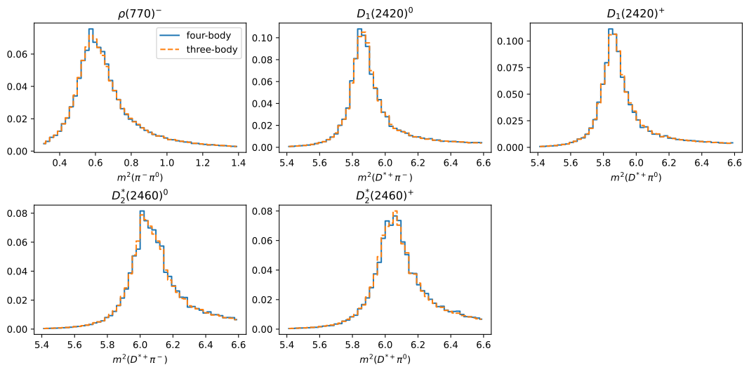
Each resonance is evaluated separately with the same helicity pattern in both models. Histograms weighted by \(wI_4\) integrate over the \(D^{*+}\) decay angles and are compared with normalized \(wI_3\) histograms from the same phase-space events.
Hide code cell source

def four_body_couplings_for(name, scale=1.0):
    latex = resonances[name].latex
    values = dict.fromkeys(four_body_couplings, 0j)
    values[
        next(c for c in four_body_couplings if c.startswith(R"H_{D^{*}(2010)^{+} \to"))
    ] = 1.0
    if subsystem_ids[name] == 1:
        values[R"H_{\rho(770)^{-} \to \pi^{-}_{0} \pi^{0}_{0}}"] = 1.0
        for helicity, weight in patterns[name].items():
            tag = HELICITY_TAG[helicity]
            key = (
                Rf"H_{{\overline{{B}}^{{0}} \to D^{{*}}(2010)^{{+}}_{{{tag}}} "
                Rf"\rho(770)^{{-}}_{{{tag}}}}}"
            )
            values[key] = scale * weight
        return values
    production = next(
        c
        for c in four_body_couplings
        if c.startswith(Rf"H_{{\overline{{B}}^{{0}} \to {{{latex}}}")
    )
    values[production] = scale
    for helicity, weight in patterns[name].items():
        prefix = Rf"H_{{{latex} \to D^{{*}}(2010)^{{+}}_{{{HELICITY_TAG[helicity]}}}"
        key = next((c for c in four_body_couplings if c.startswith(prefix)), None)
        if key is None:
            assert weight == 0
            continue
        values[key] = weight
    return values


def evaluate_four_body(name):
    four_body_function.update_parameters(four_body_couplings_for(name))
    with warnings.catch_warnings():
        warnings.simplefilter("ignore")
        return np.asarray(four_body_function(four_body_data))


variables = {1: phsp_sigma1, 2: phsp_sigma2, 3: phsp_sigma3}
labels = {
    1: R"$m^2(\pi^-\pi^0)$",
    2: R"$m^2(D^{*+}\pi^0)$",
    3: R"$m^2(D^{*+}\pi^-)$",
}
ranges = {1: (0.3, 1.4), 2: (5.4, 6.6), 3: (5.4, 6.6)}

fig, axes = plt.subplots(2, 3, figsize=(11, 5.4), layout="constrained")
deviations = []
four_body_norms = {}
for ax, name in zip(axes.ravel()[: len(DECAY_WAVE)], DECAY_WAVE, strict=True):
    subsystem = subsystem_ids[name]
    edges = np.linspace(*ranges[subsystem], 51)
    centers = (edges[1:] + edges[:-1]) / 2
    component_weights = phsp_weights * evaluate_four_body(name)
    four_body_norms[name] = float(np.mean(component_weights))
    assert np.isfinite(four_body_norms[name])
    assert four_body_norms[name] > 0
    four_body_projection, _ = np.histogram(
        variables[subsystem],
        bins=edges,
        weights=component_weights,
    )
    three_body_projection, _ = np.histogram(
        variables[subsystem],
        bins=edges,
        weights=phsp_weights * evaluate({name: 1.0}, three_body_data),
    )
    four_body_projection /= four_body_projection.sum()
    three_body_projection /= three_body_projection.sum()
    deviation = (
        np.abs(four_body_projection - three_body_projection)
        / three_body_projection.max()
    )
    deviations.append(deviation)
    ax.step(centers, four_body_projection, where="mid", label="four-body")
    ax.step(
        centers, three_body_projection, where="mid", linestyle="--", label="three-body"
    )
    ax.set(title=f"${resonances[name].latex}$", xlabel=labels[subsystem])
axes[0, 0].legend()
axes[-1, -1].axis("off")
fig.savefig("comparison.svg")
plt.show()
deviations = np.concatenate(deviations)
assert deviations.mean() < 0.03, deviations.mean()
Markdown(
    "Deviation between the normalized projections, relative to each peak: "
    f"{100 * deviations.mean():.1f}% on average and {100 * deviations.max():.1f}% at worst, "
    f"consistent with the Monte Carlo statistics of {len(phsp_weights):,} events."
)
../_images/977512d7da48643865ebcd43b7b72e06a385215acb2bfca2c13fd4aeb27ca2cc.svg

Deviation between the normalized projections, relative to each peak: 0.7% on average and 7.0% at worst, consistent with the Monte Carlo statistics of 500,000 events.

AmpForm Dalitz plot from phase space#

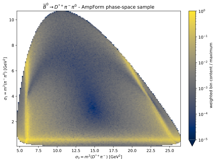
The four-body Dalitz projection uses the existing phasespace sample with the \(D^{*+}\) fixed at its pole mass. Each component is normalized by \(\langle wI_R\rangle\) to give the same input fraction as in the DPD model. The illustrative phases are applied in AmpForm’s helicity convention; no phase conversion between the two implementations is imposed.

The histogram weights are \(wI_4\), with all components evaluated coherently. Binning in \((\sigma_3,\sigma_1)\) integrates over the \(D^{*+}\) decay angles. The color scale matches the DPD plot, with each bin divided by the largest bin content.
Hide code cell source

four_body_scales = {
    name: np.sqrt(fractions[name] / norm) * np.exp(1j * np.deg2rad(phases[name]))
    for name, norm in four_body_norms.items()
}
four_body_parameters = dict.fromkeys(four_body_couplings, 0j)
for name, scale in four_body_scales.items():
    four_body_parameters.update({
        coupling: value
        for coupling, value in four_body_couplings_for(name, scale).items()
        if value != 0
    })
four_body_function.update_parameters(four_body_parameters)
four_body_values = np.asarray(four_body_function(four_body_data))
assert np.isfinite(four_body_values).all()
assert (four_body_values >= 0).all()
weighted_intensity = phsp_weights * four_body_values
sample_x_edges = np.linspace(x_edges[0], x_edges[-1], 161)
sample_y_edges = np.linspace(y_edges[0], y_edges[-1], 161)
sample_density, _, _ = np.histogram2d(
    phsp_sigma3,
    phsp_sigma1,
    bins=(sample_x_edges, sample_y_edges),
    weights=weighted_intensity,
)
np.testing.assert_allclose(sample_density.sum(), weighted_intensity.sum(), rtol=1e-10)
assert sample_density.max() > 0
sample_density /= sample_density.max()
fig, ax = plt.subplots(figsize=(7.5, 5.6), layout="constrained")
mesh = ax.pcolormesh(
    sample_x_edges,
    sample_y_edges,
    np.ma.masked_less_equal(sample_density.T, 0),
    cmap="cividis",
    norm=LogNorm(vmin=1e-5, vmax=1),
    rasterized=True,
)
ax.set(
    xlabel=projection_labels[3],
    ylabel=projection_labels[1],
    title=R"$\overline{B}^0\to D^{*+}\pi^-\pi^0$ - AmpForm phase-space sample",
)
fig.colorbar(mesh, ax=ax, label="weighted bin content / maximum", extend="min")
fig.savefig("dalitz-ampform.svg")
plt.show()
../_images/02b0177a547e245f9a1a6c65c17dd1f239d9c0a01b814d8ff7440643979080f6.svg

The comparison checks individual components. A coherent comparison also requires matching the helicity-coupling conventions of AmpForm and AmpForm-DPD.

The angular projections below use the \(D^0\) direction in the \(D^{*+}\) rest frame relative to the \(D^{*+}\) flight direction, and the angle \(\varphi\) between the \(D^{*+}\) and \(\rho^-\) decay planes. The polar distribution separates longitudinal and transverse couplings; the decay-plane distribution distinguishes the two transverse sign choices.
Hide code cell source

def boost_to_rest_frame(momentum, frame):
    mass = np.sqrt(frame[:, 0] ** 2 - (frame[:, 1:] ** 2).sum(axis=1))
    beta = -frame[:, 1:] / frame[:, 0, None]
    beta_squared = (beta**2).sum(axis=1)
    gamma = frame[:, 0] / mass
    dot = (beta * momentum[:, 1:]).sum(axis=1)
    energy = gamma * (momentum[:, 0] + dot)
    factor = (gamma - 1) * dot / beta_squared + gamma * momentum[:, 0]
    return np.column_stack([energy, momentum[:, 1:] + factor[:, None] * beta])


def unit(vector):
    return vector / np.linalg.norm(vector, axis=1)[:, None]


d_star_momentum = momenta["p0"] + momenta["p1"]
d0_direction = unit(boost_to_rest_frame(momenta["p0"], d_star_momentum)[:, 1:])
z_axis = unit(d_star_momentum[:, 1:])
cos_theta = (d0_direction * z_axis).sum(axis=1)
pion_direction = unit(
    boost_to_rest_frame(momenta["p2"], momenta["p2"] + momenta["p3"])[:, 1:]
)
decay_plane_angle = np.arccos(
    np.clip(
        (
            unit(np.cross(z_axis, d0_direction))
            * unit(np.cross(z_axis, pion_direction))
        ).sum(axis=1),
        -1,
        1,
    )
)

polar, azimuthal = {}, {}
saved_pattern = patterns["rho(770)-"]
for label, pattern in (
    ("longitudinal", {-1: 0.0, 0: 1.0, +1: 0.0}),
    ("transverse, equal signs", {-1: 1.0, 0: 0.0, +1: +1.0}),
    ("transverse, opposite signs", {-1: 1.0, 0: 0.0, +1: -1.0}),
    (Rf"$f_L={LONGITUDINAL_FRACTION}$", saved_pattern),
):
    patterns["rho(770)-"] = pattern
    weights = phsp_weights * evaluate_four_body("rho(770)-")
    if "transverse, opposite" not in label:
        polar[label] = weights
    if label.startswith("transverse"):
        azimuthal[label] = weights
patterns["rho(770)-"] = saved_pattern

fig, (left, right) = plt.subplots(1, 2, figsize=(10, 3.6), layout="constrained")
for axis, distributions, variable, edges, xlabel in (
    (left, polar, cos_theta, np.linspace(-1, 1, 21), R"$\cos\theta_{D^{*+}}$"),
    (
        right,
        azimuthal,
        decay_plane_angle,
        np.linspace(0, np.pi, 21),
        R"$\varphi$ [rad]",
    ),
):
    centers = (edges[1:] + edges[:-1]) / 2
    for label, weights in distributions.items():
        projection, _ = np.histogram(variable, bins=edges, weights=weights)
        axis.step(centers, projection / projection.sum(), where="mid", label=label)
    axis.set(xlabel=xlabel, ylabel="normalized yield")
    axis.set_ylim(0, 1.5 * axis.get_ylim()[1])
    axis.legend(fontsize="small", loc="upper center", ncols=2)
left.set_title(R"$D^{*+}$ polar angle")
right.set_title(R"$D^{*+}$-$\rho^-$ decay-plane angle")
fig.savefig("angles.svg")
plt.show()
../_images/c21c776dc5ee95548566bd3ce5b5785dc1e6e77eeb7797da8640a973942bfcd5.svg